4 Case study
4.1 A credit risk portfolio
The credit model in this section is a conditionally binomial loan portfolio model including systematic and specific portfolio risk. We refer to the Appendix A for details about the model and the generation of the simulated data. A key variable of interest is the total aggregate portfolio loss \(L = L_1 + L_2 + L_3\), where \(L_1, L_2, L_3\) are homogeneous subportfolios on a comparable scale (say, thousands of $). The dataset contains 100,000 simulations of the portfolio \(L\), the subportfolios \(L_1, L_2, L_3\) as well as the random default probabilities within each subportfolio, \(H_1, H_2, H_3\). These default probabilities represent the systematic risk within each subportfolio, while their dependence structure represents a systematic risk effect between the subportfolios. The simulated data of the credit risk portfolio are included in the SWIM package and can be accessed via data("credit_data"). A snippet of the dataset looks as follows:
##         L L1    L2  L3       H1      H2     H3
## [1,]  692  0 346.9 345 1.24e-04 0.00780 0.0294
## [2,] 1006 60 515.6 430 1.16e-03 0.01085 0.0316
## [3,] 1661  0 806.2 855 5.24e-04 0.01490 0.0662
## [4,] 1708  0 937.5 770 2.58e-04 0.02063 0.0646
## [5,]  807  0  46.9 760 8.06e-05 0.00128 0.0632
## [6,] 1159 20 393.8 745 2.73e-04 0.00934 0.0721
4.2 Stressing the portfolio loss
In this section, following a reverse sensitivity approach, we study the effects that stresses on (the tail of) the aggregate portfolio loss \(L\) have on the three subportfolios; thus assessing their comparative importance. First, we impose a \(20\%\) increase on the VaR at level \(90\%\) of the portfolio loss.
## Stressed VaR specified was 2174.25 , stressed VaR achieved is 2173.75The \(20\%\) increase was specified by setting the q_ratio argument to \(1.2\) – alternatively the argument q can be set to the actual value of the stressed VaR.
Using the function VaR_stressed, we can quantify how tail quantiles of the aggregate portfolio loss change, when moving from the baseline to the stressed model. We observe that the increase in the VaR of the portfolio loss changes more broadly its tail quantiles; thus the stress on VaR also induces an increase in ES. The implemented functions VaR_stressed and ES_stressed calculate respectively VaR and ES; the argument alpha specifies the levels of VaR and ES, respectively, while the stressed model under which the risk measures are calculated can be chosen using wCol (by default equal to 1).
VaR_stressed(object = stress.credit, alpha = c(0.75, 0.9, 0.95, 0.99),
    xCol = "L", wCol = 1, base = TRUE)
## L base L
## 75% 1506 1399
## 90% 2174 1812
## 95% 2426 2085
## 99% 2997 2671## L base L
## 90% 2535 2191As a second stress, we consider, additionally to the \(20\%\) increase in the \(\text{VaR}_{0.9}\), an increase in \(\text{ES}_{0.9}\) of the portfolio loss \(L\). When stressing VaR and ES together via stress_VaR_ES, both VaR and ES need to be stressed at the same level, here alpha = 0.9. We observe that when stressing the VaR alone, ES increases to 2535. For the second stress we want a greater impact on ES, thus we require that the stressed ES be equal to 3500. This can be achieved by specifying the argument s, which is the stressed value of ES (rather than s_ratio, the proportional increase).
stress.credit <- stress(type = "VaR ES", x = stress.credit, k = "L", alpha = 0.9,
    q_ratio = 1.2, s = 3500)
## Stressed VaR specified was 2174.25 , stressed VaR achieved is 2173.75When applying the stress function or one of its alternative versions to a SWIM object rather than to a data frame (via x = stress.credit in the example above), the result will be a new SWIM object with the new stress “appended” to existing stresses. This is convenient when large datasets are involved, as the stress function returns an object containing the original simulated data and the scenario weights. Note however, that this only works if the underlying data are exactly the same.
4.3 Analysing stressed models
The summary function provides a statistical summary of the stressed models. Choosing base = TRUE compares the stressed models with the the baseline model.
## $base
##                    L    L1     L2      L3       H1      H2     H3
## mean        1102.914 19.96 454.04 628.912 0.000401 0.00968 0.0503
## sd           526.538 28.19 310.99 319.715 0.000400 0.00649 0.0252
## skewness       0.942  2.10   1.31   0.945 1.969539 1.30834 0.9501
## ex kurtosis    1.326  6.21   2.52   1.256 5.615908 2.49792 1.2708
## 1st Qu.      718.750  0.00 225.00 395.000 0.000115 0.00490 0.0318
## Median      1020.625  0.00 384.38 580.000 0.000279 0.00829 0.0464
## 3rd Qu.     1398.750 20.00 609.38 810.000 0.000555 0.01296 0.0643
##
## $`stress 1`
##                   L    L1     L2     L3       H1      H2     H3
## mean        1193.39 20.83 501.10 671.46 0.000417 0.01066 0.0536
## sd           623.48 29.09 363.57 361.21 0.000415 0.00756 0.0285
## skewness       1.01  2.09   1.36   1.02 1.973337 1.35075 1.0283
## ex kurtosis    0.94  6.14   2.23   1.22 5.630153 2.23353 1.2382
## 1st Qu.      739.38  0.00 234.38 405.00 0.000120 0.00512 0.0328
## Median      1065.62 20.00 412.50 605.00 0.000290 0.00878 0.0483
## 3rd Qu.     1505.62 40.00 675.00 865.00 0.000578 0.01422 0.0688
##
## $`stress 2`
##                   L    L1     L2     L3       H1      H2     H3
## mean        1289.90 21.70 558.27 709.93 0.000437 0.01180 0.0566
## sd           875.90 30.57 507.78 447.30 0.000448 0.01045 0.0351
## skewness       1.90  2.17   2.10   1.57 2.090425 2.10128 1.5384
## ex kurtosis    3.67  6.74   4.79   2.80 6.203429 4.97000 2.6142
## 1st Qu.      739.38  0.00 234.38 405.00 0.000123 0.00512 0.0328
## Median      1065.62 20.00 412.50 605.00 0.000297 0.00879 0.0484
## 3rd Qu.     1505.62 40.00 675.00 875.00 0.000594 0.01439 0.0697
Note that stress 1 is the summary output corresponding to the \(20\%\) increase in the VaR, while stress 2 corresponds to the stress in both VaR and ES. The information on individual stresses can be recovered through the get_specs function, and the actual scenario weights using get_weights. Since the SWIM object stress.credit contains two stresses, the scenario weights that are returned by get_weights form a data frame consisting of two columns, corresponding to stress 1 and to stress 2, respectively.
##            type k alpha       q    s
## stress 1    VaR L   0.9 2173.75 <NA>
## stress 2 VaR ES L   0.9 2173.75 3500
# extract weights from SWIM object
w.credit <- get_weights(stress.credit)
# only plot a subset of the sceranio weights
grid <- seq(1, 100000, by = 50)
plot(credit_data[grid, 1], w.credit[grid, 1], pch = 20, xlab = "L",
ylab = "scenario weights")
plot(credit_data[grid, 1], w.credit[grid, 2], pch = 20, xlab = "L",
ylab = "scenario weights")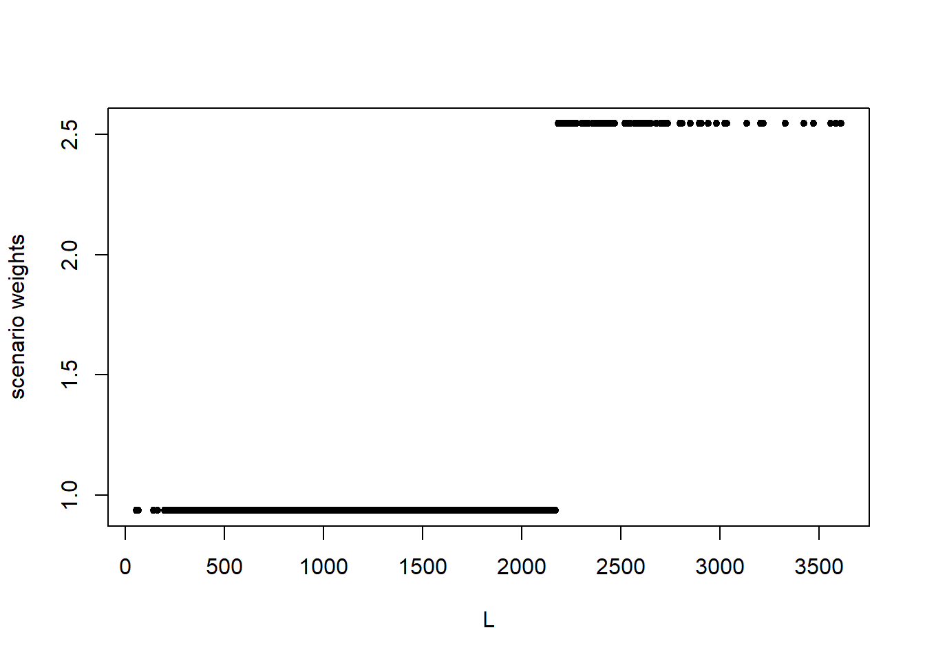
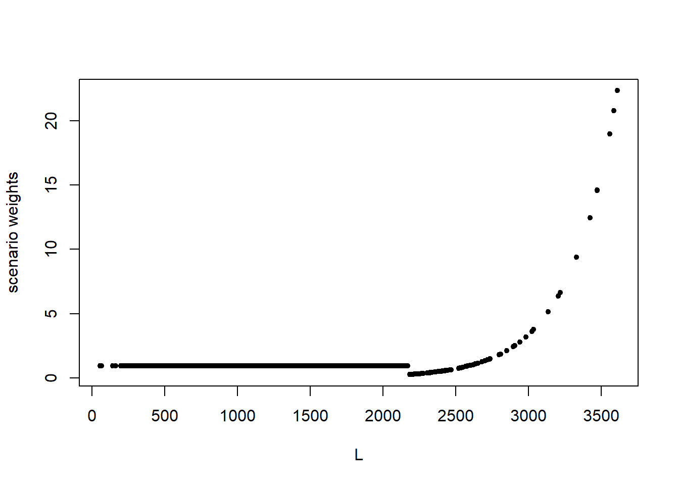
Figure 4.1: Scenario weights against the portfolio loss \(L\) for stressing VaR (left) and stressing both VaR and ES (right).
It is seen in Figure 4.1 that the weights generated to stress VaR, and VaR and ES together, follow different patterns to the weights used to stress means and standard deviations, as shown in Section 2. Recall that SWIM calculates the scenario weights such that under the stressed model the given constraints are fulfilled. Thus, an increase in the VaR and/or ES of the portfolio loss \(L\) results in large positive realisations of \(L\) being assigned higher weight. On the other hand, when the standard deviation is stressed, scenario weights are calculated that inflate the probabilities of both large positive and negative values.
4.4 Visualising stressed distributions
The change in the distributions of the portfolio and subportfolio losses, when moving from the baseline to the stressed models, can be visualised through the functions plot_hist and plot_cdf. The following figure displays the histogram of the aggregate portfolio loss under the baseline and the two stressed models. It is seen how stressing VaR and ES has a higher impact on the right tail of \(L\), compared to stressing VaR only. This is consistent with the tail-sensitive nature of the Expected Shortfall risk measure (McNeil, Frey, and Embrechts 2015).
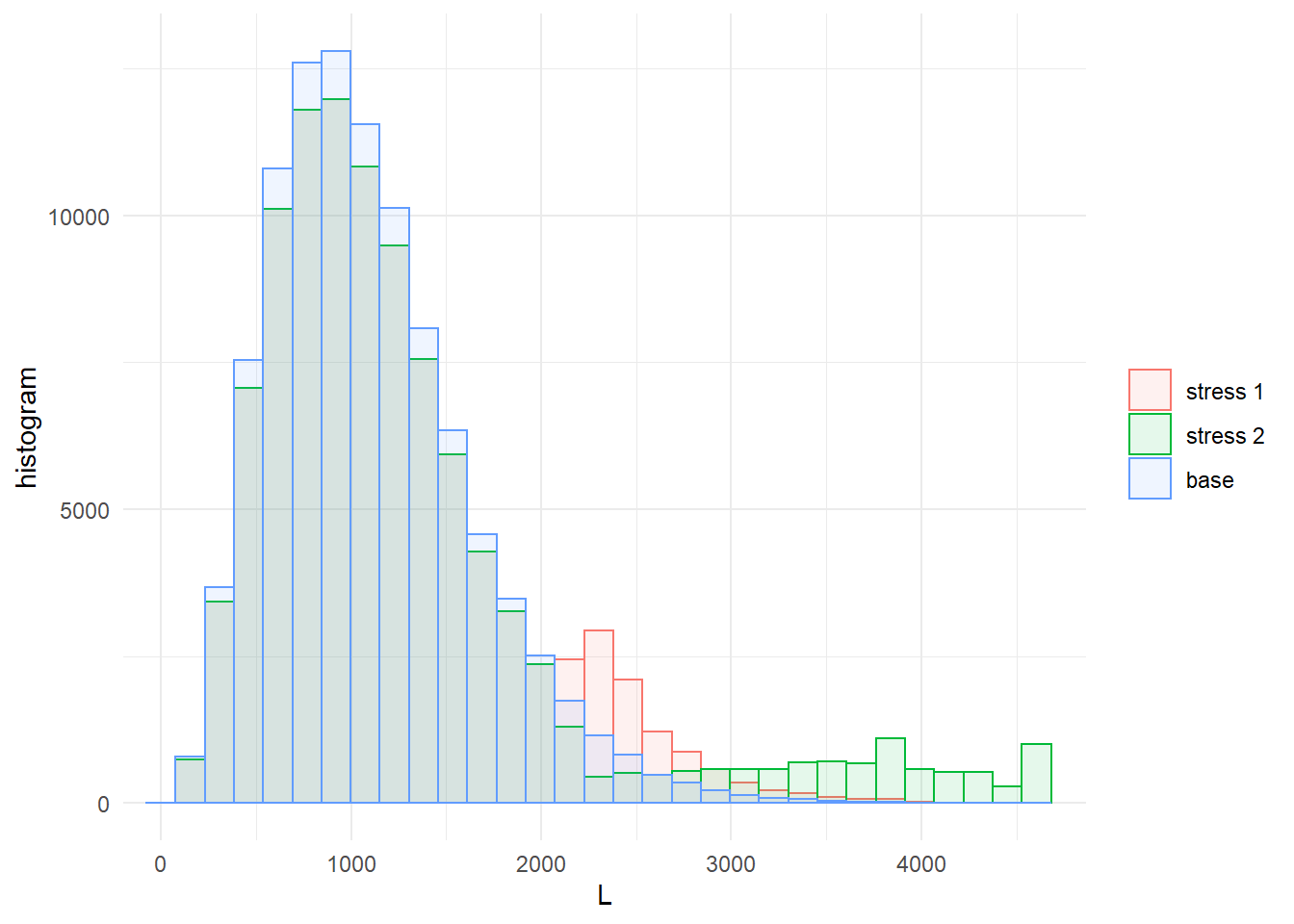
Figure 4.2: Histogram of the portfolio loss \(L\) under the baseline and the two stressed models.
The arguments xCol and wCol (with default to plot all stresses) define the columns of the data and the columns of the scenario weights, respectively, that are used for plotting. Next, we analyse the impact that stressing the aggregate loss \(L\) has on the subportfolios \(L_1,~ L_2~L_3\). Again, we use the function plot_hist and plot_cdf for visual comparison, but this time placing the distribution plots and histograms of subportfolio losses along each other via the function ggarrange (from the package ggpubr). The plots obtained from plot_hist and plot_cdf can be further personalised when specifying the argument displ = FALSE, as then the graphical functions plot_hist and plot_cdf return data frames compatible with the package ggplot2.
pL1.cdf <- plot_cdf(object = stress.credit, xCol = 2, wCol = "all", base = TRUE)
pL2.cdf <- plot_cdf(object = stress.credit, xCol = 3, wCol = "all", base = TRUE)
pL3.cdf <- plot_cdf(object = stress.credit, xCol = 4, wCol = "all", base = TRUE)

pL1.hist <- plot_hist(object = stress.credit, xCol = 2, wCol = "all", base = TRUE)
pL2.hist <- plot_hist(object = stress.credit, xCol = 3, wCol = "all", base = TRUE)
pL3.hist <- plot_hist(object = stress.credit, xCol = 4, wCol = "all", base = TRUE)

ggarrange(pL1.cdf, pL1.hist, pL2.cdf, pL2.hist, pL3.cdf, pL3.hist, ncol = 2,
    nrow = 3, common.legend = TRUE)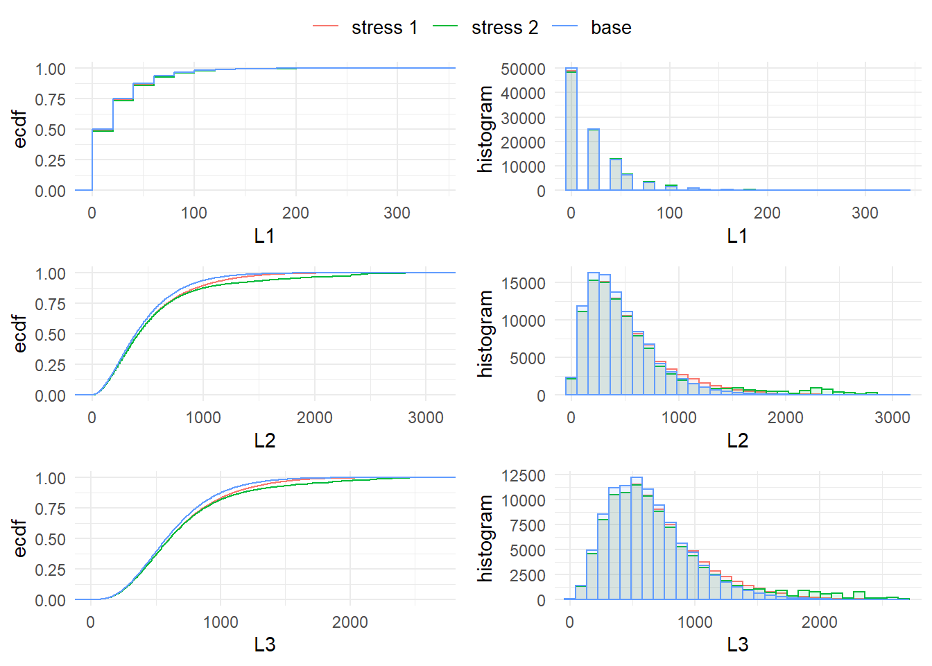
Figure 4.3: Distribution functions and histograms of the subportfolios \(L_1, L_2, L_3\) for the stresses on the VaR (stress 1) and on both the VaR and ES (stress 2) of the portfolio loss \(L\).
It is seen from both the distribution plots and the histograms in Figures 4.2 and 4.3 that the stresses have no substantial impact on \(L_1\), while \(L_2\) and \(L_3\) are more affected, indicating a higher sensitivity. The higher impact on the tails of stress 2 (on both VaR and ES) is also visible. Sensitivity measures quantifying these effects are introduced in the following subsection.
4.5 Sensitivity measures
The impact of the stressed models on the model components can be quantified through sensitivity measures. The function sensitivity includes the Kolmogorov distance, the Wasserstein distance, and the sensitivity measure Gamma; the choice of measure is by the argument type. We refer to Section 3.2 for the definitions of those sensitivity measures. The Kolmogorov distance is useful for comparing different stressed models. It is seen that stress 2 produces a more substantial distortion to the baseline distribution of \(L\) compared to stress 1.
##     stress       type      L
## 1 stress 1 Kolmogorov 0.0607
## 2 stress 2 Kolmogorov 0.0748
We now rank the sensitivities of model components by the measure Gamma, for each stressed model. Consistently with what the distribution plots showed, \(L_2\) is the most sensitive subportfolio, followed by \(L_3\) and \(L_1\). The respective default probabilities \(H_1,H_2,H_3\) are similarly ranked.
##     stress  type    L1    L2    L3    H1    H2    H3
## 1 stress 1 Gamma 0.150 0.819 0.772 0.196 0.811 0.767
## 2 stress 2 Gamma 0.113 0.734 0.639 0.171 0.708 0.636
Using the sensitivity function we can analyse whether the sensitivity of the joint subportfolio \(L_1 + L_3\) exceeds the sensitivity of the (most sensitive) subportfolio \(L_2\). This can be accomplished by specifying, through the argument f, a list of functions applicable to the columns k of the dataset. By setting xCol = NULL only the transformed data is considered. The sensitivity measure of functions of columns of the data is particularly useful when high dimensional models are considered, providing a way to compare the sensitivity of blocks of model components.
##     stress  type    f1
## 1 stress 1 Gamma 0.783
We observe that the sensitivity of \(L_1 + L_3\) is larger than the sensitivity to either \(L_1\) and \(L_3\), reflecting the positive dependence structure of the credit risk portfolio. Nonetheless, subportfolio \(L_2\) has not only the largest sensitivity compared to \(L_1\) and \(L_3\) but also a higher sensitivity than the combined subportfolios \(L_1 + L_3\).
The importance_rank function, having the same structure as the sensitivity function, returns the ranks of the sensitivity measures. This function is particularly useful when several risk factors are involved.
##     stress  type L1 L2 L3 H1 H2 H3
## 1 stress 1 Gamma  6  1  3  5  2  4
4.6 Constructing more advanced stresses
4.6.1 Sensitivity of default probabilities
From the preceding analysis, it transpires that the subportfolios \(L_2\) and \(L_3\) are, in that order, most responsible for the stress in the portfolio loss, under both stresses considered. Furthermore, most of the sensitivity seems to be attributable to the systematic risk components \(H_2\) and \(H_3\), reflected by their high values of the Gamma measure. To investigate this, we perform another stress, resulting once again in a \(20\%\) increase in \(\text{VaR}(L)\), but this time fixing some elements of the distribution of \(H_2\). Specifically, in addition to the \(20\%\) increase in \(\text{VaR}(L)\), we fix the mean and the \(75\%\) quantile of \(H_2\) to the same values as in the baseline model. This set of constraints is implemented via the function stress_moment.
# 90% VaR of L under the baseline model
VaR.L <- quantile(x = credit_data[, "L"], prob = 0.9, type = 1)
# 75th quantile of H2 under the baseline model
q.H2 <- quantile(x = credit_data[, "H2"], prob = 0.75, type = 1)
# columns to be stressed (L, H2, H2)
k.stressH2 = list(1, 6, 6)
# functions to be applied to columns
f.stressH2 <- list(
                 # indicator function for L, for stress on VaR
                 function(x)1 * (x <= VaR.L * 1.2),
                 # mean of H2
                 function(x)x,
                 # indicator function for 75th quaantile of H2
                 function(x)1 * (x <= q.H2))
# new values for the 90% VaR of L, mean of H2, 75th quantile of H2
m.stressH2 = c(0.9, mean(credit_data[, "H2"]), 0.75)
stress.credit <- stress_moment(x = stress.credit, f = f.stressH2, k = k.stressH2,
                               m = m.stressH2)
Using the summary function, we verify that the distribution of \(H_2\) under the new stress has unchanged mean and 75th quantile. Then we compare the sensitivities of the subportfolio losses under all three stresses applied.
## $base
##                  H2
## mean        0.00968
## sd          0.00649
## skewness    1.30834
## ex kurtosis 2.49792
## 1st Qu.     0.00490
## Median      0.00829
## 3rd Qu.     0.01296
##
## $`stress 3`
##                  H2
## mean        0.00968
## sd          0.00706
## skewness    1.39135
## ex kurtosis 2.26506
## 1st Qu.     0.00453
## Median      0.00786
## 3rd Qu. 0.01296## stress type L1 L2 L3
## 1 stress 1 Gamma 0.1501 0.8195 0.772
## 2 stress 2 Gamma 0.1131 0.7336 0.639
## 3 stress 3 Gamma 0.0102 0.0203 0.366It is seen that, by fixing part of the distribution of \(H_2\), the importance ranking of the subportfolios changes, with \(L_2\) now being significantly less sensitive than \(L_3\). This confirms, in the credit risk model, the dominance of the systematic risk reflected in the randomness of default probabilities.
4.6.2 Stressing tails of subportfolios
Up to now, we have considered the impact of stressing the aggregate portfolio loss on subportfolios. Now, following a forward sensitivity approach, we consider the opposite situation: stressing the subportfolio losses and monitoring the impact on the aggregate portfolio loss \(L\). First, we impose a stress requiring a simultaneous \(20\%\) increase in the 90th quantile of the losses in subportfolios \(L_2\) and \(L_3\). Note that the function stress_VaR (and stress_VaR_ES) allow to stress the VaR and/or the ES of only one model component. Thus, to induce a stress on the 90th quantiles of \(L_2\) and \(L_3\), we use the function stress_moments and interpret the quantile constraints as moment constraints, via \(E(1_{L_2 \leq \text{VaR}^W(L_2)})\) and \(E(1_{L_3 \leq \text{VaR}^W(L_3)})\), respectively, where \(\text{VaR}^W = \text{VaR} \cdot 1.2\) denotes the VaRs in the stressed model.
# VaR of L2 and L3, respectively
VaR.L2 <- quantile(x = credit_data[, "L2"], prob = 0.9, type = 1)
VaR.L3 <- quantile(x = credit_data[, "L3"], prob = 0.9, type = 1)
#stressing VaR of L2 and L3
f.stress <- list(function(x)1 * (x <= VaR.L2 * 1.2),
                 function(x)1 * (x <= VaR.L3 * 1.2))
stress.credit.L2L3 <- stress_moment(x = credit_data, f = f.stress, k = list(3, 4),
                                    m = c(0.9, 0.9))
#impact on portfolio tail
VaR_stressed(stress.credit.L2L3, alpha = c(0.75, 0.9, 0.95, 0.99), xCol = "L",
             base = TRUE)
## L base L
## 75% 1556 1399
## 90% 2086 1812
## 95% 2423 2085
## 99% 3072 2671It is seen how the stressing of subportfolios \(L_2\) and \(L_3\) has a substantial impact on the portfolio loss. Given the importance of dependence for the distribution of the aggregate loss of the portfolio, we strengthen this stress further, by additionally requiring that the frequency of joint high losses from \(L_2\) and \(L_3\) is increased. Specifically, we require the joint exceedance probability to be \(P^W(L_2 > VaR^W(L_2),~ L_3 > VaR^W(L_3)) = 0.06\), which is almost doubling the corresponding probability in the last stressed model, which was equal to 0.0308.
# probability of joint exceendance under the baseline model
mean(1 * (credit_data[, "L2"] > VaR.L2 * 1.2) * (credit_data[, "L3"] >
    VaR.L3 * 1.2))
## [1] 0.00865# probability of joint exceendance under the stressed model
mean(get_weights(stress.credit.L2L3) * (credit_data[, "L2"] > VaR.L2 *
1.2) * (credit_data[, "L3"] > VaR.L3 * 1.2))## [1] 0.0308# additionally stress joint exceedance probability of L2 and L3
f.stress.joint <- c(f.stress, function(x) 1 * (x[1] > VaR.L2 * 1.2) * (x[2] >
VaR.L3 * 1.2))
stress.credit.L2L3 <- stress_moment(x = stress.credit.L2L3, f = f.stress.joint,
k = list(3, 4, c(3, 4)), m = c(0.9, 0.9, 0.06))We analyse the impact the stresses of the tail of the subportfolios \(L_2\) and \(L_3\) have on the aggregate portfolio \(L\). For this, we plot in Figure 4.4 the quantile of the aggregate portfolio under the baseline model (blue), under the stress on the tail of \(L_2\) and \(L_3\) (red), and under the additional stress on the joint tail of \(L_2\) and \(L_3\) (green).
# stressed quantiles
VaR.level <- seq(0.75, 0.99, by = 0.003)
VaR.stress1 <- VaR_stressed(stress.credit.L2L3, alpha = VaR.level, xCol = "L",
    wCol = 1, base = TRUE)
VaR.stress2 <- VaR_stressed(stress.credit.L2L3, alpha = VaR.level, xCol = "L",
    wCol = 2, base = FALSE)

plot(VaR.level, VaR.stress1[, 2], col = "blue", type = "l", xlab = "quantile levels",
    ylab = "Quantiles of L under different models")
lines(VaR.level, VaR.stress1[, 1], col = "red")
lines(VaR.level, VaR.stress2, col = "darkgreen")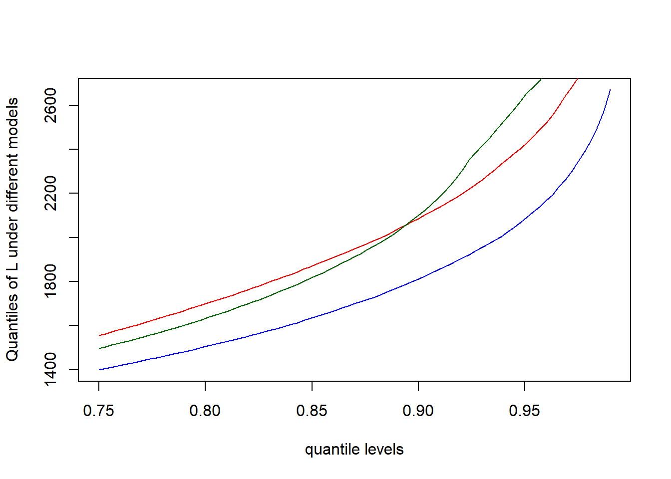
Figure 4.4: Quantiles of the aggregate loss \(L\) under the baseline (blue), the stress on the tails of \(L_2\) and \(L_3\) (red), and the additional stress on the joint tail of \(L_2\) and \(L_3\) (green).
The results and the plots indicate that the additional stress on joint exceedances of subportfolios, increases the tail quantiles of \(L\) even further, demonstrating the importance of (tail-)dependence in portfolio risk management.