2 What is SWIM?
2.1 Sensitivity testing and scenario weights
The purpose of SWIM is to enable sensitivity analysis of models implemented in a Monte Carlo simulation framework, by distorting (stressing) some of the models’ components and monitoring the resulting impact on quantities of interest. To clarify this idea and explain how SWIM works, we first define the terms used. By a model, we mean a set of \(n\) (typically simulated) realisations from a vector of random variables \((X_1,\dots,X_d)\), along with scenario weights \(W\) assigned to individual realisations, as shown in the table below. Hence each of of the columns 1 to \(d\) corresponds to a random variable, called a model component, while each row corresponds to a scenario, that is, a state of the world.
| \(X_1\) | \(X_2\) | \(\dots\) | \(X_d\) | \(W\) |
|---|---|---|---|---|
| \(x_{11}\) | \(x_{21}\) | \(\dots\) | \(x_{d1}\) | \(w_1\) |
| \(x_{12}\) | \(x_{22}\) | \(\dots\) | \(x_{d2}\) | \(w_2\) |
| \(\vdots\) | \(\vdots\) | \(\ddots\) | \(\vdots\) | \(\vdots\) |
| \(x_{1n}\) | \(x_{2n}\) | \(\dots\) | \(x_{dn}\) | \(w_n\) |
Each scenario has a scenario weight, shown in the last column, such that, scenario \(i\) has probability \(\frac{w_i}{n}\) of occurring. Scenario weights are always greater or equal than zero and have an average of 1. When all scenario weights are equal to 1, such that the probability of each scenario is \(\frac 1 n\) (the standard Monte Carlo framework), we call the model a baseline model – consequently weights of a baseline model will never be explicitly mentioned. When scenario weights are not identically equal to 1, such that some scenarios are more weighted than others, we say that we have a stressed model.
The scenario weights make the joint distribution of model components under the stressed model different, compared to the baseline model. For example, under the baseline model, the expected value of \(X_1\) and the cumulative distribution function of \(X_1\), at threshold \(t\), are respectively given by:
\[ E(X_1)=\frac 1 n \sum_{i=1}^nx_{1i},\quad F_{X_1}(t)= P(X_1\leq t)=\frac 1 n \sum_{i=1}^n \mathbf 1 _{x_{1i}\leq t}, \]
where \(\mathbf 1 _{x_{1i}\leq t}=1\) if \(x_{1i}\leq t\) and \(0\) otherwise. For a stressed model with scenario weights \(W\), the expected value \(E^W\) and cumulative distribution function \(F^W\) become:
\[ E^W(X_1)=\frac 1 n \sum_{i=1}^n w_i x_{1i},\quad F_{X_1}^W(t)=P^W(X_1\leq t)=\frac 1 n \sum_{i=1}^n w_i \mathbf 1 _{x_{1i}\leq t}. \]
Similar expressions can be derived for more involved quantities, such as higher (joint) moments and quantiles.
The logic of stressing a model with SWIM then proceeds as follows. An analyst or modeller is supplied with a baseline model, in the form of a matrix of equiprobable simulated scenarios of model components. The modeller wants to investigate the impact of a change in the distribution of, say, \(X_1\). To this effect, she chooses a stress on the distribution of \(X_i\), for example requiring that \(E^W(X_1)=m\); we then say that she is stressing \(X_1\) and, by extension, the model. Subsequently, SWIM calculates the scenario weights such that the stress is fulfilled and the distortion to the baseline model induced by the stress is as small as possible; specifically the Kullback-Leibler divergence (or relative entropy) between the baseline and stressed models is minimised. (See Section 3.1 for more detail on the different types of possible stresses and the corresponding optimisation problems). Once scenario weights are obtained, they can be used to determine the stressed distribution of any model component or function of model components. For example, for scenario weights \(W\) obtained through a stress on \(X_1\), we may calculate
\[ E^W(X_2)=\frac 1 n\sum_{i=1}^n w_i x_{2i},\quad E^W(X_1^2+X_2^2)=\frac 1 n \sum_{i=1}^n w_i \left(x_{1i}^2+ x_{2i}^2 \right). \]
Through this process, the modeller can monitor the impact of the stress on \(X_1\) on any other random variable of interest. It is notable that this approach does not necessitate generating new simulations from a stochastic model. As the SWIM approach requires a single set of simulated scenarios (the baseline model) it offers a clear computational benefit.
2.2 An introductory example
Here, through an example, we illustrate the basic concepts and usage of SWIM for sensitivity analysis. More advanced usage of SWIM and options for constructing stresses are demonstrated in Sections 3 and 4. We consider a simple portfolio model, with the portfolio loss defined by \(Y=Z_1+Z_2+Z_3\). The random variables \(Z_1,Z_2,Z_3\) represent normally distributed losses, with \(Z_1\sim N(100,40^2)\), \(Z_2\sim Z_3\sim N(100,20^2)\). \(Z_1\) and \(Z_2\) are correlated, while \(Z_3\) is independent of \((Z_1,Z_2)\). Our purpose in this example is to investigate how a stress on the loss \(Z_1\) impacts on the overall portfolio loss \(Y\). First we derive simulated data from the random vector \((Z_1,Z_2,Z_3,Y)\), forming our baseline model.
set.seed(0)
# number of simulated scenarios
n.sim <- 10 ^ 5
# correlation between Z1 and Z2
r <- 0.5
# simulation of Z1  and Z2
# constructed as a combination of independent standard normals U1, U2
U1 <- rnorm(n.sim)
U2 <- rnorm(n.sim)
Z1 <- 100 + 40 * U1
Z2 <- 100 + 20 * (r * U1 + sqrt(1 - r ^ 2) * U2)
# simulation of Z3
Z3 <- rnorm(n.sim, 100, 20)
# portfolio loss Y
Y <- Z1 + Z2 + Z3
# data of baseline model
dat <- data.frame(Z1, Z2, Z3, Y)
Now we introduce a stress to our baseline model. For our first stress, we require that the mean of \(Z_1\) is increased from 100 to 110. This is done using the stress function, which generates as output the SWIM object str.mean. This object stores the stressed model, i.e. the realisations of the model components and the scenario weights. In the function call, the argument k = 1 indicates that the stress is applied on the first column of dat, that is, on the realisations of the random variable \(Z_1\).
library(SWIM)
str.mean <- stress(type = "mean", x = dat, k = 1, new_means = 110)
summary(str.mean, base = TRUE)
## $base
## Z1 Z2 Z3 Y
## mean 1.0e+02 99.9404 99.9843 299.9811
## sd 4.0e+01 19.9970 19.9819 56.6389
## skewness -6.1e-04 0.0012 -0.0025 -0.0023
## ex kurtosis -1.1e-02 -0.0090 -0.0126 -0.0094
## 1st Qu. 7.3e+01 86.4745 86.4816 261.6121
## Median 1.0e+02 99.9866 100.0091 300.0548
## 3rd Qu. 1.3e+02 113.3957 113.4934 338.2670
##
## $`stress 1`
## Z1 Z2 Z3 Y
## mean 110.0000 102.4437 99.9828 312.4265
## sd 40.0333 19.9954 19.9762 56.6173
## skewness -0.0024 -0.0015 -0.0049 -0.0037
## ex kurtosis -0.0050 -0.0032 -0.0155 -0.0012
## 1st Qu. 82.9984 88.9771 86.4815 274.2200
## Median 110.0759 102.4810 99.9954 312.5039
## 3rd Qu. 136.9310 115.8744 113.5019 350.6120The summary function, applied to the SWIM object str.mean, shows how the distributional characteristics of all random variables change from the baseline to the stressed model. In particular, we see that the mean of \(Z_1\) changes to its required value, while the mean of \(Y\) also increases. Furthermore there is a small impact on \(Z_2\), due to its positive correlation to \(Z_1\).
Beyond considering the standard statistics evaluated via the summary function, stressed probability distributions can be plotted. In Figure 2.1 we show the impact of the stress on the cumulative distribution functions (cdf) of \(Z_1\) and \(Y\). It is seen how the stressed cdfs are lower than the original (baseline) ones. Loosely speaking, this demonstrates that the stress has increased (in a stochastic sense) both random variables \(Z_1\) and \(Y\). While the stress was on \(Z_1\), the impact on the distribution of the portfolio \(Y\) is clearly visible.
# refer to variable of interest by name...
plot_cdf(str.mean, xCol = "Z1", base = TRUE)
# ... or column number
plot_cdf(str.mean, xCol = 4, base = TRUE)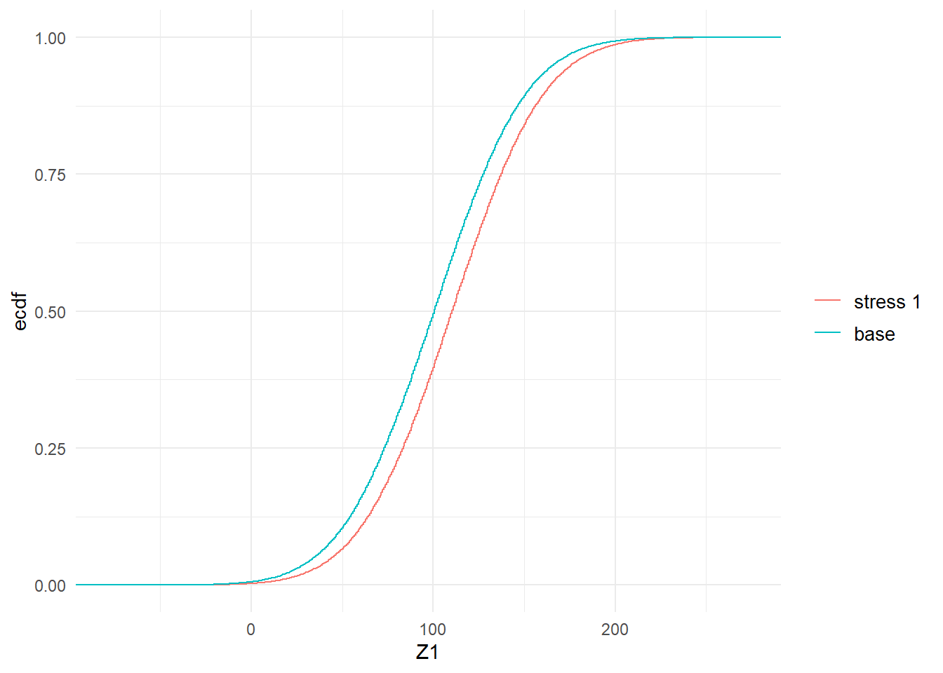
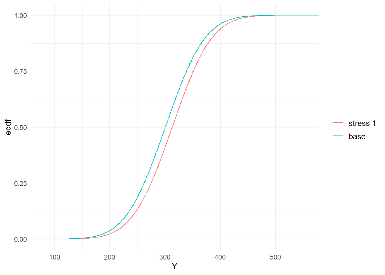
Figure 2.1: Baseline and stressed empirical distribution functions of model components \(Z_1\) (left) and \(Y\) (right), subject to a stress on the mean of \(Z_1\).
The scenario weights, given their central role, can be extracted from a SWIM object. In Figure 2.2, the scenario weights from str.mean are plotted against realisations from \(Z_1\) and \(Y\) respectively. It is seen how the weights are increasing in the realisations from \(Z_1\). This is a consequence of the weights’ derivation via a stress on the model component \(Z_1\). The increasingness shows that those scenarios for which \(Z_1\) is largest are assigned a higher weight. The relation between scenario weights and \(Y\) is still increasing (reflecting that high outcomes of \(Y\) tend to receive higher weights), but no longer deterministic (showing that \(Y\) is not completely driven by changes in \(Z_1\)).
# extract weights from stressed model
w.mean <- get_weights(str.mean)
plot(Z1[1:5000], w.mean[1:5000], pch = 20, xlab = "Z1", ylab = "scenario weights")
plot(Y[1:5000], w.mean[1:5000], pch = 20, xlab = "Y", ylab = "scenario weights")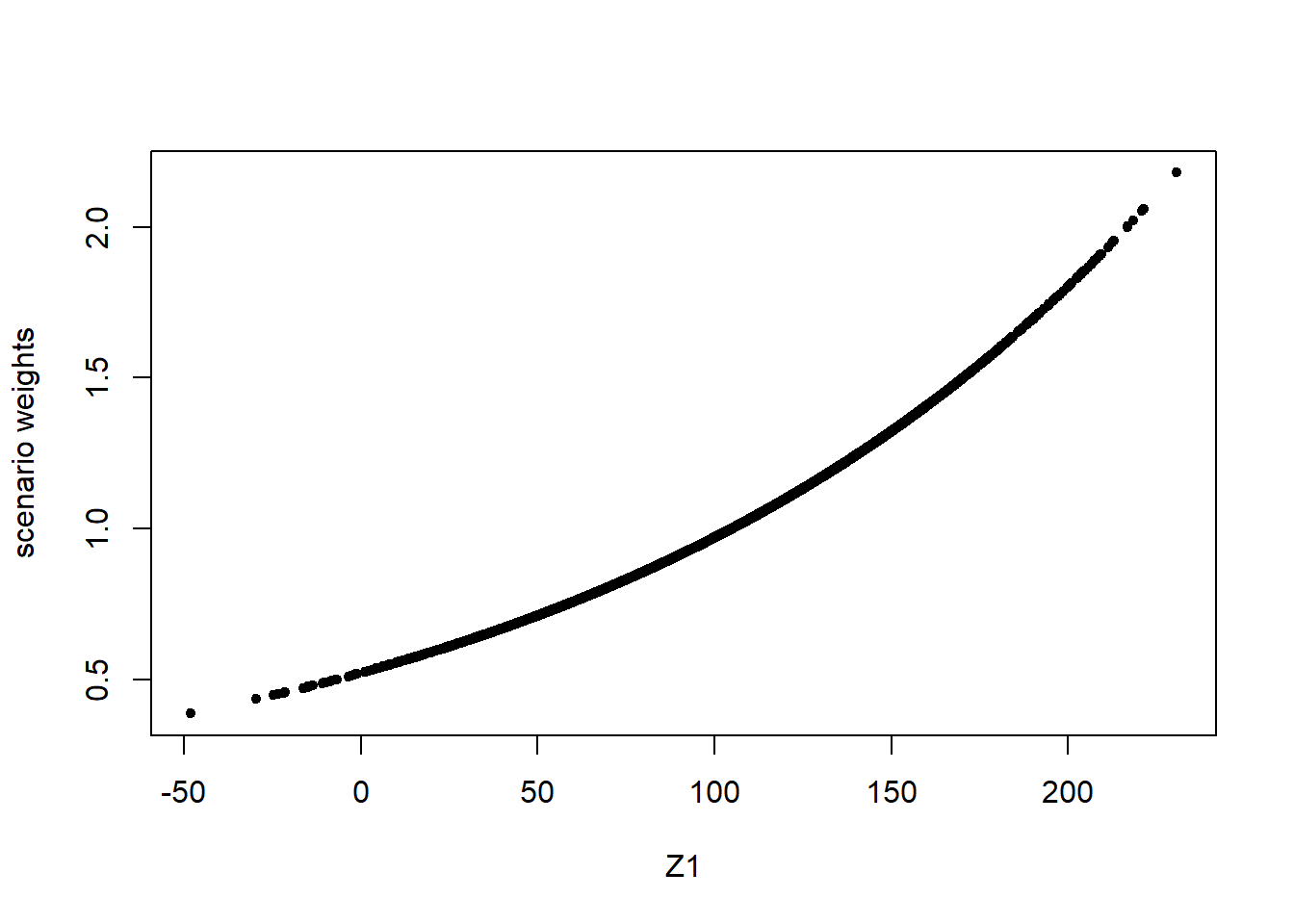
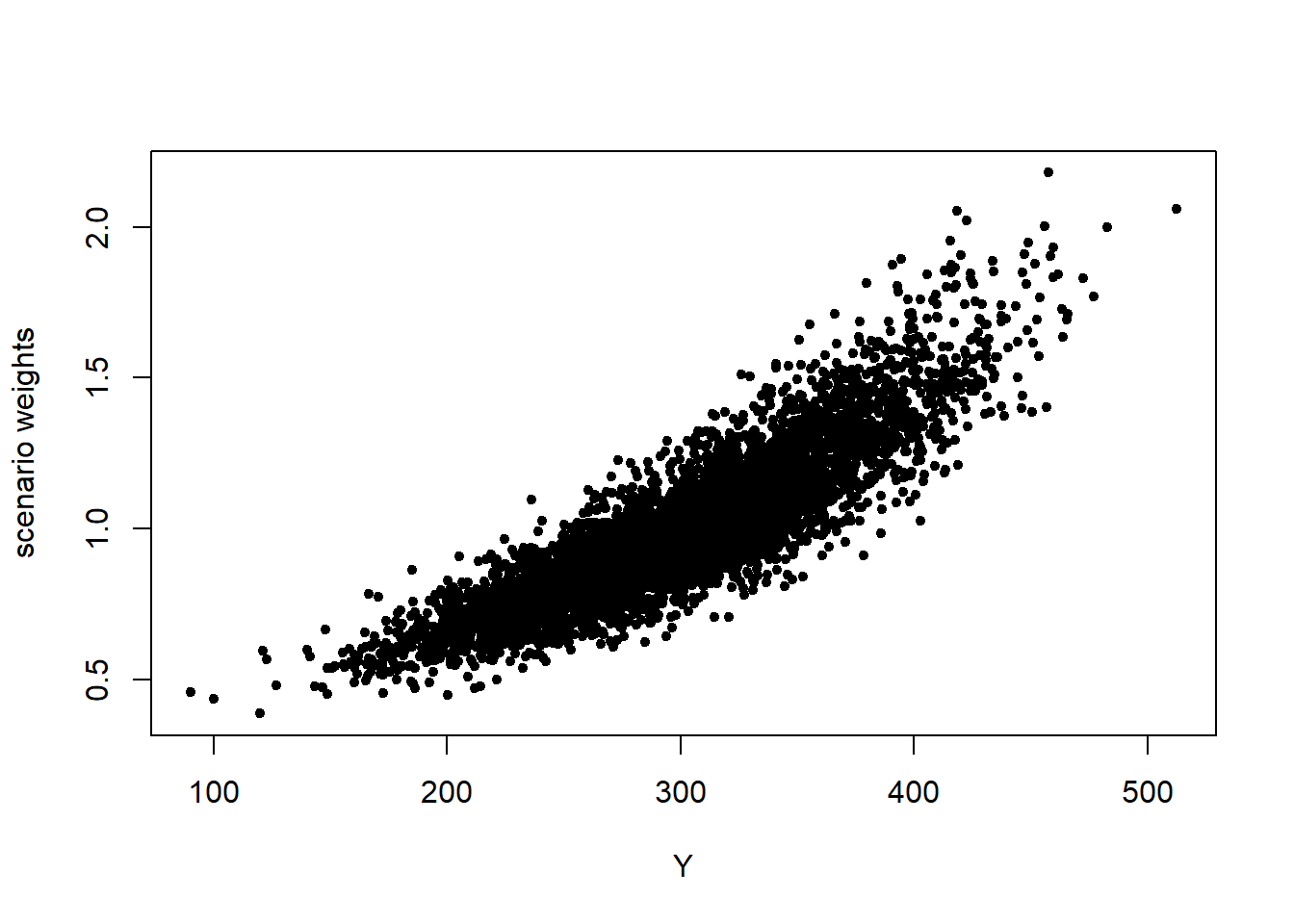
Figure 2.2: Scenario weights against observations of model components \(Z_1\) (left) and \(Y\) (right), subject to a stress on the mean of \(Z_1\).
The stress to the mean of \(Z_1\) did not impact the volatility of either \(Z_1\) or \(Y\), as can be seen by the practically unchanged standard deviations in the output of summary(str.mean). Thus, we introduce an alternative stress that keeps the mean of \(Z_1\) fixed at 100, but increases its standard deviation from 40 to 50. This new stress is seen to impact the standard deviation of the portfolio loss \(Y\).
str.sd <- stress(type = "mean sd", x = dat, k = 1, new_means = 100, new_sd = 50)
summary(str.sd, base = FALSE)
## $`stress 1`
## Z1 Z2 Z3 Y
## mean 100.0000 99.941 99.9782 299.9187
## sd 50.0005 21.349 19.9800 67.9233
## skewness -0.0027 0.007 -0.0034 0.0049
## ex kurtosis -0.0556 -0.033 -0.0061 -0.0427
## 1st Qu. 66.0964 85.495 86.4822 253.7496
## Median 100.1290 99.974 100.0455 299.9766
## 3rd Qu. 133.7733 114.301 113.4701 345.9159Furthermore, in Figure 2.3, we compare the baseline and stressed cdfs of \(Z_1\) and \(Y\), under the new stress on \(Z_1\). The crossing of probability distribution reflects the increase in volatility.
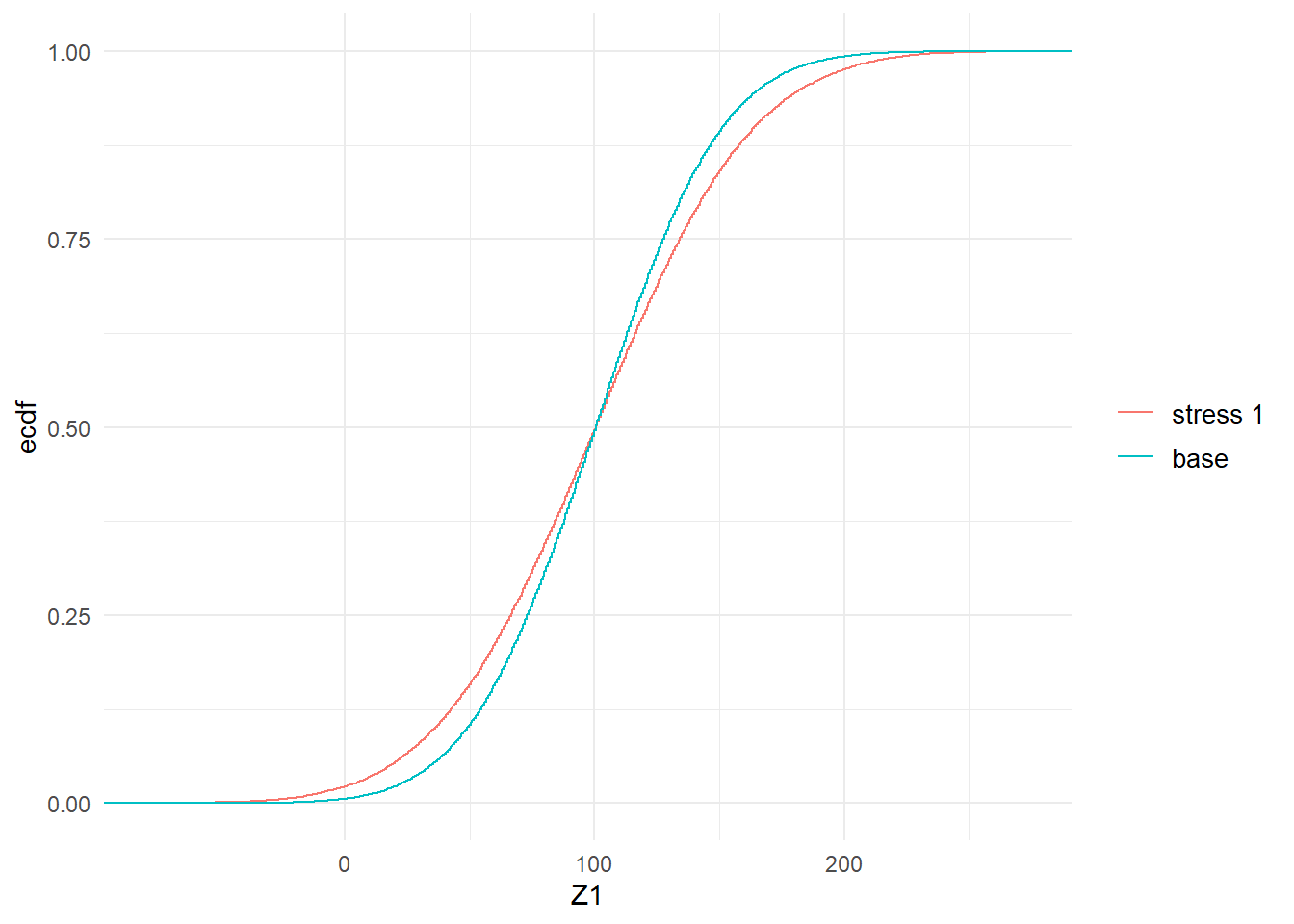
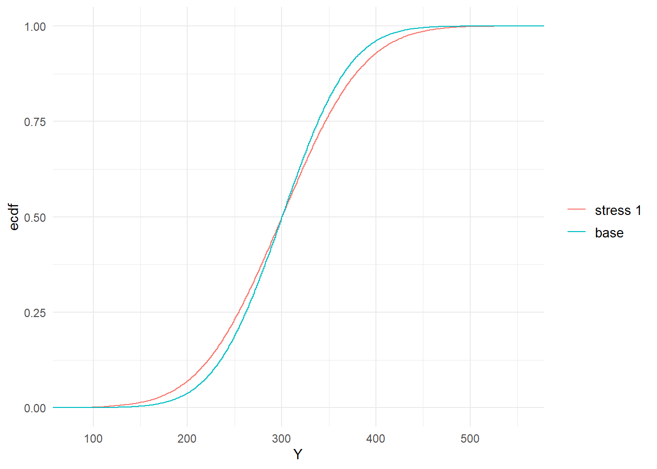
Figure 2.3: Baseline and stressed empirical distribution functions of model components \(Z_1\) (left) and \(Y\) (right), subject to a stress on the standard deviation of \(Z_1\).
The different way in which a stress on the standard deviation of \(Z_1\) impacts on the model, compared to a stress on the mean, is reflected by the scenario weights. Figure 2.4 shows the pattern of the scenario weights and how, when stressing standard deviations, higher weight is placed on scenarios where \(Z_1\) is extreme, either much lower or much higher than its mean of 100.
w.sd <- get_weights(str.sd)
plot(Z1[1:5000], w.sd[1:5000], pch = 20, xlab = "Z1", ylab = "scenario weights")
plot(Y[1:5000], w.sd[1:5000], pch = 20, xlab = "Y", ylab = "scenario weights")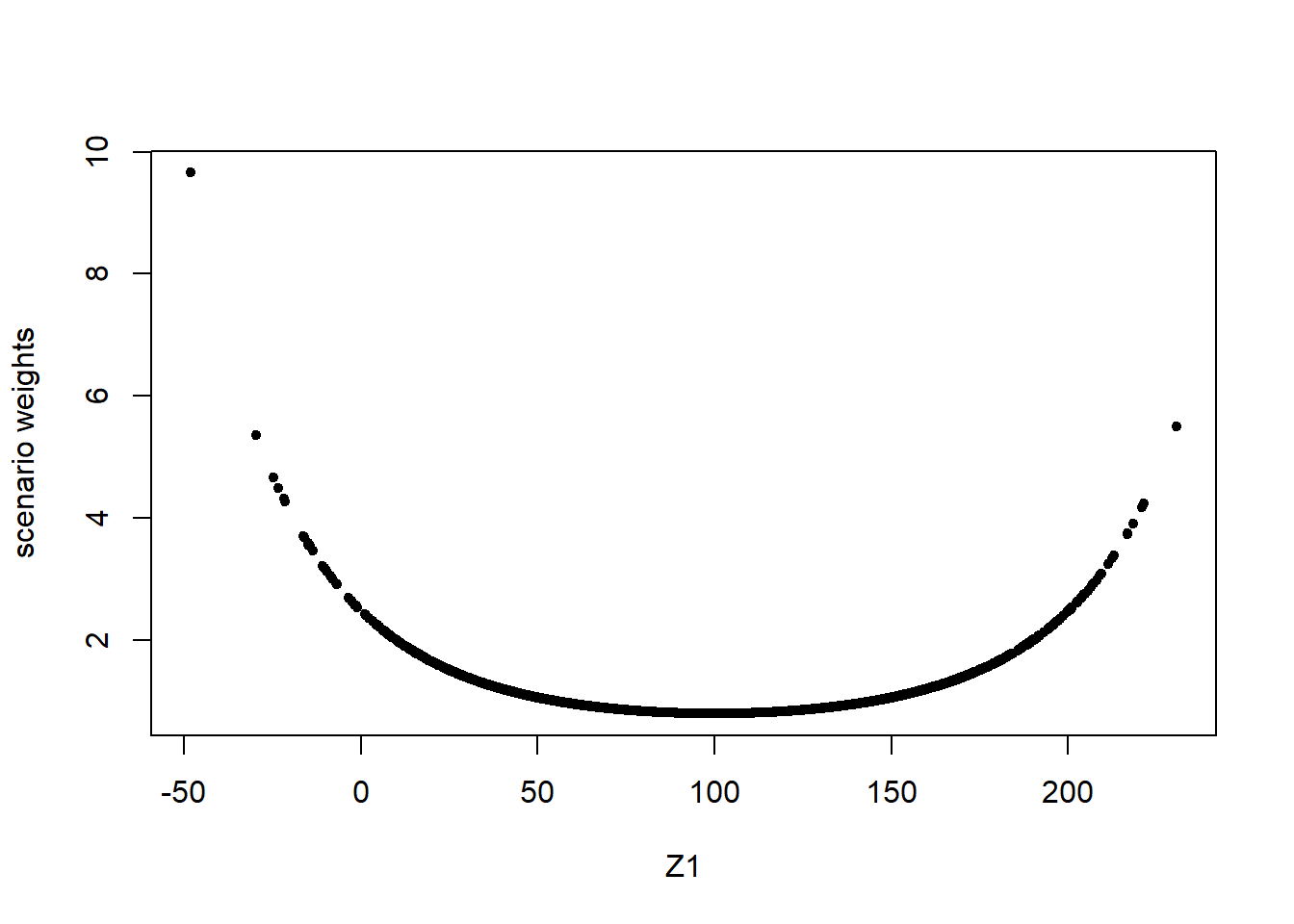
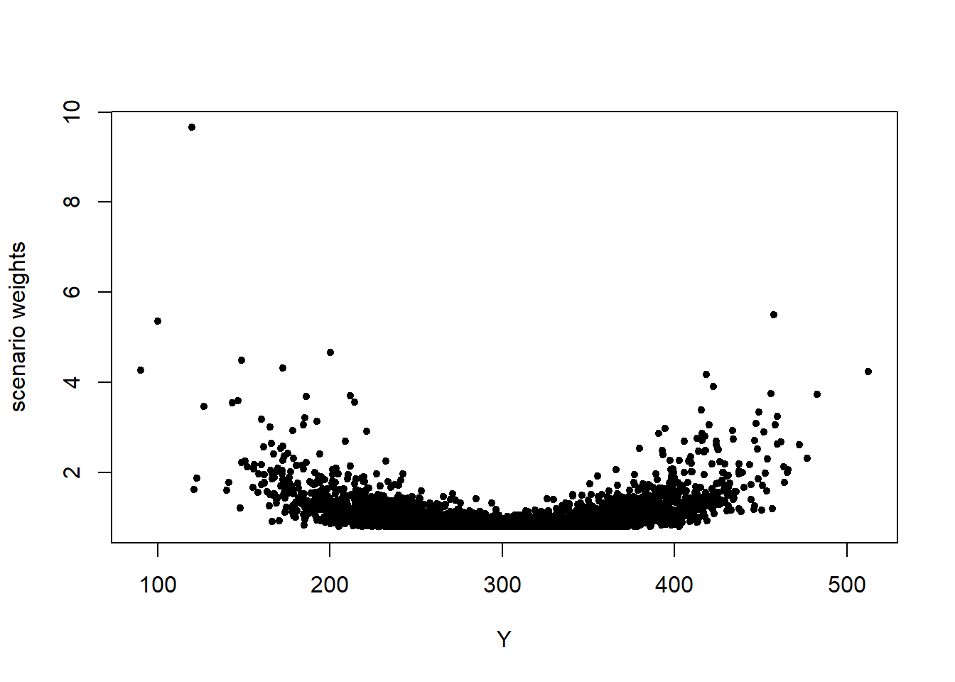
Figure 2.4: Scenario weights against observations of model components \(Z_1\) (left) and \(Y\) (right), subject to a stress on the standard deviation of \(Z_1\).
Finally we ought to note that not all stresses that one may wish to apply are feasible. Assume for example that we want to increase the mean of \(Z_1\) from 100 to 300, which exceeds the maximum realisation of \(Z_1\) in the baseline model. Then, clearly, no set of scenario weights can be found that produce a stress that yields the required mean for \(Z_1\); consequently an error message is produced.
## Error in stress_moment(x = x, f = means, k = as.list(k), m = new_means, :
Values in m must be in the range of f(x)## [1] 273